42 chart data labels excel

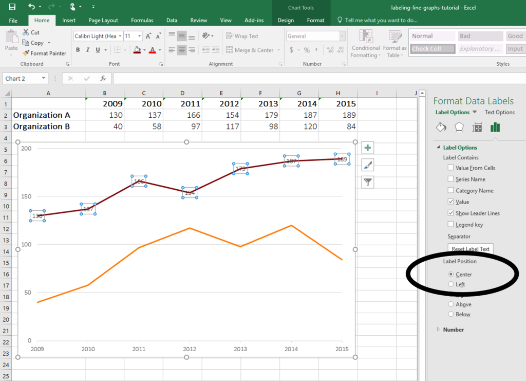
How To Add Data Labels In Excel - danielsadventure.info Click on the arrow next to data labels to change the position of where the labels are in relation to the bar chart. Add A Label (Form Control) Click Developer, Click Insert, And Then Click Label. You can now configure the label as required — select the content of. To format data labels in excel, choose the set of data labels to format. How to add a line in Excel graph: average line, benchmark, etc. Select the last data point on the line and add a data label to it as discussed in the previous tip. Click on the label to select it, then click inside the label box, delete the existing value and type your text: ... How to make trend line upto few bars in excel chart. I do not want trend line for entire bars what ever available in chart ...

support.microsoft.com › en-us › officeAdd or remove data labels in a chart - support.microsoft.com You can add data labels to show the data point values from the Excel sheet in the chart. This step applies to Word for Mac only: On the View menu, click Print Layout . Click the chart, and then click the Chart Design tab.

Chart data labels excel

Custom Chart Data Labels In Excel With Formulas - How To Excel At Excel Follow the steps below to create the custom data labels. Select the chart label you want to change. In the formula-bar hit = (equals), select the cell reference containing your chart label's data. In this case, the first label is in cell E2. Finally, repeat for all your chart laebls. How do you label data points in Excel? - Profit claims 1. Right click the data series in the chart, and select Add Data Labels > Add Data Labels from the context menu to add data labels. 2. Click any data label to select all data labels, and then click the specified data label to select it only in the chart. 3. Adding Data Labels to Your Chart (Microsoft Excel) - ExcelTips (ribbon) To add data labels in Excel 2013 or later versions, follow these steps: Activate the chart by clicking on it, if necessary. Make sure the Design tab of the ribbon is displayed. (This will appear when the chart is selected.) Click the Add Chart Element drop-down list. Select the Data Labels tool.

Chart data labels excel. How to change Axis labels in Excel Chart - A Complete Guide Enter the labels you want to use in the Axis label range box, separated by commas. In the Axis label range box, enter arbitrary labels separated by commas. Click OK to confirm the chart axis labels change. Method-3: Using another Data Source Repeat steps 1 to 3 of Method 2. Select the cells containing the new value range to use the X-axis. How to Change Axis Labels in Excel (3 Easy Methods) Firstly, right-click the category label and click Select Data > Click Edit from the Horizontal (Category) Axis Labels icon. Then, assign a new Axis label range and click OK. Now, press OK on the dialogue box. Finally, you will get your axis label changed. That is how we can change vertical and horizontal axis labels by changing the source. How to Make a Gantt Chart in PowerPoint (6 Steps) | ClickUp To edit your Gantt chart in PowerPoint, follow these steps: Click the "Format" tab and choose "Chart Tools". Select the drop-down arrow next to "Chart Layouts," then click " Insert Blank Chart". Click on the "Format Axis" button (the one with a horizontal line) and choose an axis type from the menu that appears (e.g., linear ... Excel Pie Chart Multiple Data Labels - Multiplication Chart Printable Excel Pie Chart Multiple Data Labels - You can create a multiplication chart in Stand out simply by using a template. You will find a number of samples of themes and learn how to file format your multiplication graph or chart using them. Below are a few tips and tricks to make a multiplication chart.

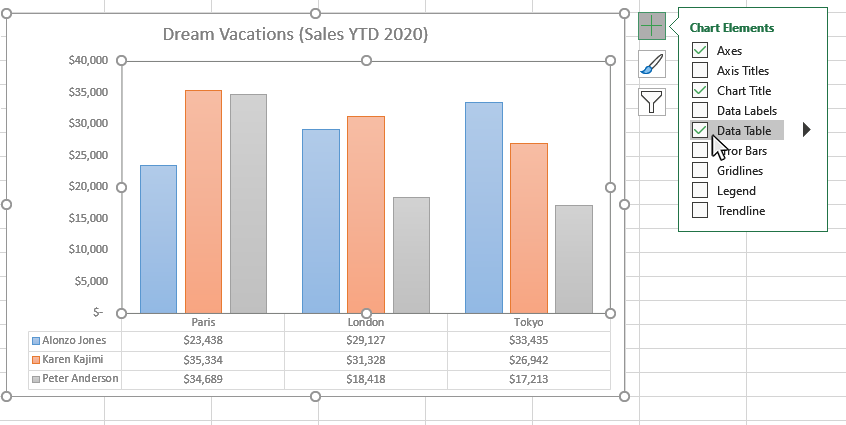
Data Labels in Excel Pivot Chart (Detailed Analysis) 7 Suitable Examples with Data Labels in Excel Pivot Chart Considering All Factors 1. Adding Data Labels in Pivot Chart 2. Set Cell Values as Data Labels 3. Showing Percentages as Data Labels 4. Changing Appearance of Pivot Chart Labels 5. Changing Background of Data Labels 6. Dynamic Pivot Chart Data Labels with Slicers 7. What are the Chart elements in Excel | Easy Learn Methods After creating a chart, you can add new chart elements in excel like chart titles, axis titles, legends, data labels, grid lines, etc. Many of them are optional and you always can remove or add them according to your needs, default displays the most essential elements when creating the chart. You can also change the formatting of existing ones. How to Add Total Values to Stacked Bar Chart in Excel The following chart will be created: Step 4: Add Total Values. Next, right click on the yellow line and click Add Data Labels. The following labels will appear: Next, double click on any of the labels. In the new panel that appears, check the button next to Above for the Label Position: Next, double click on the yellow line in the chart. Pie Chart in Excel - Inserting, Formatting, Filters, Data Labels Click on the Instagram slice of the pie chart to select the instagram. Go to format tab. (optional step) In the Current Selection group, choose data series "hours". This will select all the slices of pie chart. Click on Format Selection Button. As a result, the Format Data Point pane opens.

› solutions › excel-chatHow to Insert Axis Labels In An Excel Chart | Excelchat The method below works in the same way in all versions of Excel. How to add horizontal axis labels in Excel 2016/2013 . We have a sample chart as shown below; Figure 2 – Adding Excel axis labels. Next, we will click on the chart to turn on the Chart Design tab; We will go to Chart Design and select Add Chart Element; Figure 3 – How to label ... › excel › how-to-add-total-dataHow to Add Total Data Labels to the Excel Stacked Bar Chart Apr 03, 2013 · Step 4: Right click your new line chart and select “Add Data Labels” Step 5: Right click your new data labels and format them so that their label position is “Above”; also make the labels bold and increase the font size. Step 6: Right click the line, select “Format Data Series”; in the Line Color menu, select “No line” Step 7 ... › excel › excel-chart-data-rangeModify Excel Chart Data Range | CustomGuide The new data needs to be in cells adjacent to the existing chart data. Rename a Data Series. Charts are not completely tied to the source data. You can change the name and values of a data series without changing the data in the worksheet. Select the chart; Click the Design tab. Click the Select Data button. Remove Chart Data Labels With Specific Value Remove Chart Data Labels With Specific Value Chris Newman There may be times when you would like to de-clutter your data labels so that smaller or zero values are removed from your Excel Chart. In this article, you will find a few examples of how you can accomplish this with VBA code. The two methodologies covered are:

How-to Use Data Labels from a Range in an Excel Chart - Excel ...

How to add text labels on Excel scatter chart axis - Data Cornering Add dummy series to the scatter plot and add data labels. 4. Select recently added labels and press Ctrl + 1 to edit them. Add custom data labels from the column "X axis labels". Use "Values from Cells" like in this other post and remove values related to the actual dummy series. Change the label position below data points.

microsoft excel - Prevent two sets of labels from overlapping ...

How to Add Two Data Labels in Excel Chart (with Easy Steps) Select the data labels. Then right-click your mouse to bring the menu. Format Data Labels side-bar will appear. You will see many options available there. Check Category Name. Your chart will look like this. Now you can see the category and value in data labels. Read More: How to Format Data Labels in Excel (with Easy Steps) Things to Remember

How to Make Pie Chart with Labels both Inside and Outside ...

› how-to-create-excel-pie-chartsHow to Make a Pie Chart in Excel & Add Rich Data Labels to ... Sep 08, 2022 · In this article, we are going to see a detailed description of how to make a pie chart in excel. One can easily create a pie chart and add rich data labels, to one’s pie chart in Excel. So, let’s see how to effectively use a pie chart and add rich data labels to your chart, in order to present data, using a simple tennis related example.

Add Data Labels for Total to Stacked Columns in #Excel | wmfexcel

How to add data labels from different columns in an Excel chart? To add data labels, right-click the set of data in the chart, then pick the Add Data Labels option in Add Data Labels from the context menu. This will bring up a new window. Step 6. This is the data label that is currently shown in the chart. Step 7. If you click any data label, then all data labels will be selected.

Solved: Data labels overlap with Bar chart area - Microsoft ...

How to Show Percentages in Stacked Column Chart in Excel? Follow the below steps to show percentages in stacked column chart In Excel: Step 1: Open excel and create a data table as below. Step 2: Select the entire data table. Step 3: To create a column chart in excel for your data table. Go to "Insert" >> "Column or Bar Chart" >> Select Stacked Column Chart. Step 4: Add Data labels to the chart.

Apply Custom Data Labels to Charted Points - Peltier Tech

› documents › excelHow to add data labels from different column in an Excel chart? This method will guide you to manually add a data label from a cell of different column at a time in an Excel chart. 1.Right click the data series in the chart, and select Add Data Labels > Add Data Labels from the context menu to add data labels.

How to Place Labels Directly Through Your Line Graph in ...

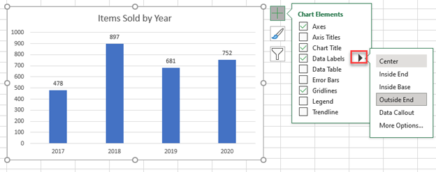
How to add data labels in excel to graph or chart (Step-by-Step) 1. Select a data series or a graph. After picking the series, click the data point you want to label. 2. Click Add Chart Element Chart Elements button > Data Labels in the upper right corner, close to the chart. 3. Click the arrow and select an option to modify the location. 4.

Add or remove data labels in a chart

DataLabels object (Excel) | Microsoft Learn Use the DataLabels method of the Series object to return the DataLabels collection. The following example sets the number format for data labels on series one on chart sheet one. VB With Charts (1).SeriesCollection (1) .HasDataLabels = True .DataLabels.NumberFormat = "##.##" End With

Adding Data Labels to Your Chart (Microsoft Excel)

DataLabel object (Excel) | Microsoft Learn Use DataLabels ( index ), where index is the data-label index number, to return a single DataLabel object. The following example sets the number format for the fifth data label in series one in embedded chart one on worksheet one. VB Worksheets (1).ChartObjects (1).Chart _ .SeriesCollection (1).DataLabels (5).NumberFormat = "0.000"

Two-Level Axis Labels (Microsoft Excel)

Excel: How to Create a Bubble Chart with Labels - Statology Step 3: Add Labels. To add labels to the bubble chart, click anywhere on the chart and then click the green plus "+" sign in the top right corner. Then click the arrow next to Data Labels and then click More Options in the dropdown menu: In the panel that appears on the right side of the screen, check the box next to Value From Cells within ...

Custom data labels in a chart

How to Add Data Labels to Scatter Plot in Excel (2 Easy Ways) - ExcelDemy 2 Methods to Add Data Labels to Scatter Plot in Excel 1. Using Chart Elements Options to Add Data Labels to Scatter Chart in Excel 2. Applying VBA Code to Add Data Labels to Scatter Plot in Excel How to Remove Data Labels 1. Using Add Chart Element 2. Pressing the Delete Key 3. Utilizing the Delete Option Conclusion Related Articles

Change color of data label placed, using the 'best fit ...

support.microsoft.com › en-us › officeEdit titles or data labels in a chart - support.microsoft.com You can also place data labels in a standard position relative to their data markers. Depending on the chart type, you can choose from a variety of positioning options. On a chart, do one of the following: To reposition all data labels for an entire data series, click a data label once to select the data series.

Excel charts: add title, customize chart axis, legend and ...

Adding Data Labels to Your Chart (Microsoft Excel) - ExcelTips (ribbon) To add data labels in Excel 2013 or later versions, follow these steps: Activate the chart by clicking on it, if necessary. Make sure the Design tab of the ribbon is displayed. (This will appear when the chart is selected.) Click the Add Chart Element drop-down list. Select the Data Labels tool.

How to Place Labels Directly Through Your Line Graph in ...

How do you label data points in Excel? - Profit claims 1. Right click the data series in the chart, and select Add Data Labels > Add Data Labels from the context menu to add data labels. 2. Click any data label to select all data labels, and then click the specified data label to select it only in the chart. 3.